Testing MCMC code: the prior reproduction test
Markov Chain Monte Carlo (MCMC) is a class of algorithms for sampling from probability distributions. These are very useful algorithms, but it’s easy to go wrong and obtain samples from the wrong probability distribution. What’s more, it won’t be obvious if the sampler fails, so we need ways to check whether it’s working correctly.
This post is mainly aimed at MCMC practitioners and describes a powerful MCMC test called the Prior Reproduction Test (PRT). I’ll go over the context of the test, then explain how it works (and give some code). I’ll then explain how to tune it and discuss some limitations.
Why should we test MCMC code ?
There are two main ways MCMC can fail: either the chain doesn’t mix or the sampler targets the wrong distribution. We say that a chain mixes if it explores the target distribution in its entirety without getting stuck or avoiding a certain subset of the space. To check that a chain mixes, we use diagnostics such as running the chain for a long time and examining the trace plots, calculating the \(\hat{R}\) (or potential scale reduction factor), and using the multistart heuristic. See the Handbook of MCMC for a good overview of these diagnostics. These help check that the chain converges to a distribution.
However the target distribution of the sampler may not be the correct one. This could be due to a bug in the code or an error in the maths (for example the Hastings correction in the Metropolis-Hastings algorithm could be wrong). To test the software, we can do tests such as unit tests which check that individual functions act like they should. We can also do integration tests (testing the entire software rather than just a component). One such test is to try to recover simulated values (as recommended by the Stan documentation): generate data given some “true” parameters (using your data model) and then fit the model using the sampler. The true parameter that should be within the credible interval (loosely within 2 standard deviations of it). This checks that the sampler can indeed recover the true parameter.
However this test is only a “sanity check” and doesn’t check whether samples are truly from the target distribution. What’s needed here is a goodness of fit (GoF) test. As doing a GoF test for arbitrarily complex posterior distributions is hard, the PRT reduces the problem to testing that some samples are from the prior rather than the posterior. I had trouble finding books or articles written about this (a similar version of this test is described by Cook, Gelman, and Rubin here, but they don’t call it PRT); if you know of any references let me know! [Update April 2021: Nianqiao (Phyllis) Ju has pointed out some references for this in the literature: Geweke (2004) describes the same method. Other similar approaches: Simulation Based Calibration (2020), and Testing MCMC Code (2014)].
I know of this test from my PhD supervisor Yvo Pokern who learnt it from another researcher during his postdoc. From talking to other researchers, it seems that this method has often been transmitted by word of mouth rather than from textbooks.
The Prior Reproduction Test
The prior reproduction test runs as follows: sample from the prior \(\theta_0 \sim \pi_0\), generate data using this prior sample \(X \sim p(X|\theta_0)\), and run the to-be-tested sampler long enough to get an independent sample from the posterior \(\theta_p \sim \pi(\theta|X)\). If the code is correct, the samples from the posterior should be distributed according to the prior. One can repeat this procedure to obtain many samples \(\theta_p\) and test whether they are distributed according to the prior.
Here is the test in Python (code available on Github). First we define the observation operator \(\mathcal{G}\)) (the mapping from parameter to data, in this case simply the identity) along with the log-likelihood, log-prior, and log-posterior. So here our data is simply sampled from a Gaussian with mean 5 and standard deviation 3.
def G(theta):
	"""
	G(theta): observation operator. Here it's just the identity function, but it could
	be a more complicated model.
	"""
	return theta

# data noise:
sigma_data = 3

def build_log_likelihood(data_array):
	"Builds the log_likelihood function given some data"
	def log_likelihood(theta):
		"Data model: y = G(theta) + eps"
		return - (0.5)/(sigma_data**2)
			* np.sum([(elem - G(theta))**2 for elem in data_array])
	return log_likelihood

def log_prior(theta):
	"uniform prior on [0, 10]"
	if not (0 < theta < 10):
		return -9999999
	else:
		return np.log(0.1)

def build_log_posterior(log_likelihood):
	"Builds the log_posterior function given a log_likelihood"
	def log_posterior(theta):
		return log_prior(theta) + log_likelihood(theta)
	return log_posterior
We want to the test the code for a Metropolis sampler with Gaussian proposal (given in the MCMC module), so we run the PRT for it (the following code is in the run_PRT() function in PRT.py):
results = []
B = 200

for elem in range(B):
	# sample from prior
	sam_prior = np.random.uniform(0,10)

	# generate data points using the sampled prior
	data_array = G(sam_prior) + np.random.normal(loc=0, scale=sigma_data, size=10)

	# build the posterior function
	log_likelihood = build_log_likelihood(data_array=data_array)
	log_posterior = build_log_posterior(log_likelihood)

	# define the sampler
	ICs = {'theta': 1}
	sd_proposal = 20
	mcmc_sampler = MHSampler(log_post=log_posterior, ICs=ICs, verbose=0)
	# add a Gaussian proposal
	mcmc_sampler.move = GaussianMove(ICs, cov=sd_proposal)

	# Get a posterior sample.
	# Let the sampler run for 200 iterations to make sure it's independent from the initial condition
	mcmc_sampler.run(n_iter=200, print_rate=300)
	last_sample = mcmc_sampler.all_samples.iloc[-1].theta

	# store the results. Keep the posterior sample as well as the prior that generated the data
	results.append({'posterior': last_sample, 'prior': sam_prior})
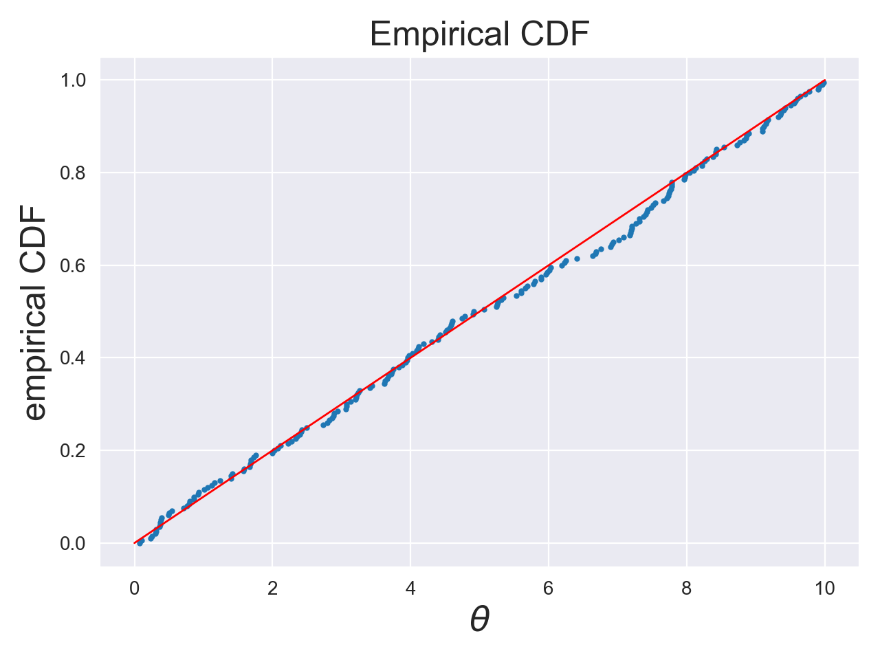
We then check that the posterior samples are uniformly distributed (i.e. the same as the prior) (see figure 1). Here we do this by eye, but we could have done this more formally (for example using the Kolmogorov-Smirnov test).
Tuning the PRT
Notice how we let the sampler run for 200 iterations to make sure that the posterior sample we get is independent of the initial condition (mcmc_sampler.run(n_iter=200, print_rate=300)). The number of iterations used needs to be tuned to the sampler; if it’s slow then you’ll need more samples. This means that a slowly mixing sampler will cause the PRT to become more computationally expensive. We also needed to tune the proposal variance in the Gaussian proposal (called sd_proposal); ideally this will be a good tuning for any dataset generated in the PRT, but this may not always be the case. Sometimes the sampler needs hand tuning for each generated dataset; in this case it may also be too expensive to run the entire test. We’ll see later what other tests we can do in this case.
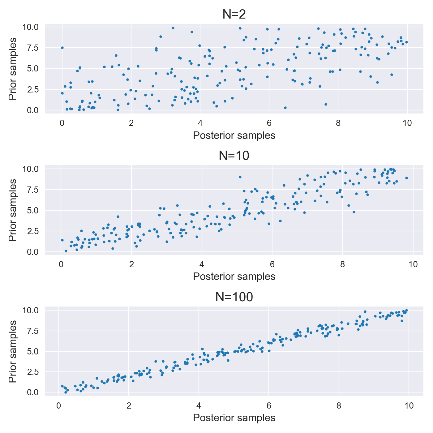
Finally, how do we choose the amount of data to generate (here we chose 10 data points)? Consider 2 extremes: if we choose too much data then the posterior will have a very low variance and will be centred around the true parameter. So almost any posterior sample we obtain will be close to the true parameter (which we sampled from the prior), and so the PRT will (trivially) produce samples from the prior. This doesn’t test the statistical properties of the sampler, but rather tests that the posterior is centred around the true parameter. In the other extreme case, if we have too little data the likelihood will have a weak effect on the posterior, which will then essentially be the prior. The MCMC sampler will then sample from a distribution that is very close to prior, and again the PRT becomes weaker. We therefore need to choose somewhere in the middle.
To tune the amount of data to generate we can plot the posterior vs the prior samples from the PRT as we can see in figure 2 below. Ideally there is a nice amount of variation around the line y=x as in the middle plot (for N=10 data points). In the other two case the PRT will trivially recover prior samples and not test the software properly.
Limitations and alternatives
In some cases however it’s not possible to run the PRT. The likelihood may be too computationally expensive; it might require solving numerically a differential equation for example. It’s also possible that the proposal distribution needs to be tuned for each dataset. In this case you have to tune the proposal manually at each iteration of the PRT.
A way to deal with these problems is to only test conditionals of the posterior (in the case of higher dimensional posteriors). For example if the posterior is \(\pi(\theta_1, \theta_2)\), then run the test on \(\pi(\theta_1 | \theta_2)\). In some cases this can solve the problem of needing to retune the proposal distribution for every dataset. This also helps with the problem of expensive likelihoods, as the dimension of the conditional posterior is lower than the original one. Less samples are then needed to run the test.
Another very simple alternative is to use the sampler to sample from the prior (so simply commenting out the likelihood function in the posterior). This completely bypasses the problem of expensive likelihoods and the need to retune the proposal at every step. This test checks that the MCMC proposal is correct (the Hastings correction for example), so is good for testing complicated proposals. However if the proposal needed to sample from the prior is qualitatively different from the proposal needed to sample from the posterior, then it’s not a useful test.
As mentioned in the introduction, the PRT reduces to testing goodness of fit of prior samples, the idea being that this is easier to test as prior distributions are often chosen for their simplicity. One can of course test goodness of fit on the MCMC samples directly (without the PRT) using a method such as the Kernel Goodness-of-fit test. This avoids the problems discussed above, but it requires gradients of the log target density, whereas the PRT makes no assumptions about the target distribution.
Conclusions
The Prior Reproduction Test is a powerful way to test MCMC code but can be expensive computationally. This test - along with its simplified versions described above - can be included in an arsenal of diagnostics to check that MCMC samples are from the correct distribution.
Code to reproduce the figures is on Github
Thanks to Heiko Strathmann and Lea Goetz for useful feedback on this post