A few years ago Bob Carpenter wrote a fantastic post on how why ensemble methods cannot work in high dimensions. He explains how high dimensions proposals that interpolate and extrapolate among samples are unlikely to fall in the typical set, causing the sampler to fail. During my PhD I worked on sampling problems with infinite-dimension parameters (ie: functions) and intractible gradients. After reading Bob’s post I always wondered if there was a way around this problem.

I finally got round to working on this idea and wrote a paper (arXiv) with Robert J Webber about an ensemble method for function spaces (ie: infinite dimensional parameters) which works very well. This sampler is aimed at sampling functions when gradients are unavailable (due to a black-box code base or discontinuous likelihoods for example).

So does that mean that Bob was wrong about ensemble samplers? Of course not; it rather turns out that not all high dimensional distributions are the same. Namely: there is sometimes a low-dimensional subset of parameter space that represents all the “interesting bits” of the posterior that you can focus on.

After giving a problem to motivate function space samplers, I’ll introduce the functional ensemble sampler (FES). I’ll then discuss what this means for using gradient-free samplers such as ensemble samplers in high dimensional spaces. You can skip directly to the discussion section for a reply to Bob’s post, which can be read independently of the description of the FES algorithm.

Functional ensemble sampler

A motivational problem

Consider the 1D advection equation, a linear hyperbolic PDE. This PDE models how a quantity - such as the density of fluid - propagates through 1D domain over time. This PDE is a special case of more complicated nonlinear PDEs that arise in fluid dynamics, acoustic, motorway traffic flow, and many more applications. The equation is given as follows (with subscripts denoting partial differentiation):

\[\rho_t + c \rho_x = 0\]

Here \(\rho\) is density and \(c \in \mathcal{R}\) is the wave speed of the fluid. We define the initial condition \(\rho_0 \equiv \rho_0(x)\) to be the state of density of the fluid at time \(t=0\). This linear PDE simply advects the initial condition to the right or left of the domain depending on the sign of \(c\).

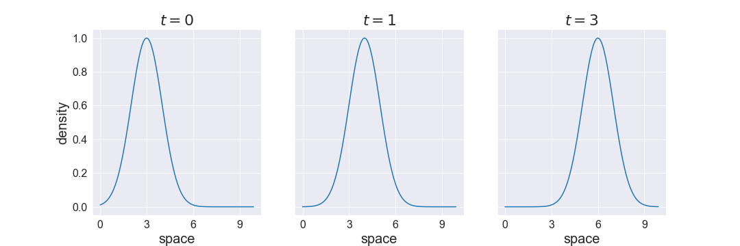
So the solution can be written as \(\rho(x,t) = \rho_0(x-ct)\). The following figure shows how an initial density profile is advected (ie: transported) to the right with wavespeed \(c=1\).

An inverse problem might then be: given some noisy observations of flow at a few locations (these could correspond to detectors along a pipe for example), recover the initial condition as well as the wave speed of the fluid. Note that flow is the product of density and speed: \(q = \rho c\). Using this relation and the solution of the PDE above, we can write the data model for a detector at location \(x\) measuring flow at time \(t\):

\[q(x, t) = c\rho_0(x-ct) + \xi\]

with \(\xi \sim \mathcal{N}(0,1)\) the observational noise.

To solve this inverse problem, we need to set a prior on both parameters, so we choose a uniform prior for the wave speed, and a Gaussian Process (GP) prior for the initial condition.

Sampling from function spaces

pCN

The most basic gradient free sampler defined on function space is preconditioned Crank Nicholson (pCN) (see this paper for an overview). This sampler makes the following simple proposal, with \(u\) current MCMC sample, \(\beta \in (0,1)\) and \(\xi \sim \mathcal{N}(0, \Sigma_0)\) a sample from the prior:

\[\tilde{u} = \sqrt{1-\beta^2}u + \beta \xi\]

The acceptance rate for this sampler is independent of dimension so is well suited for sampling function (though in practice they’re discretisations of functions). However this sampler can mix slowly if the posterior is very different from the prior, for example if some of the components of the function are very correlated or multimodal.

FES

The idea of the functional ensemble sampler is to do an eigenfunction expansion of the prior and use that to isolate a low-dimensional subspace that includes the “difficult bit” of the posterior. This means that we can represent functions \(u\) in this space by truncating the eigenexpansion to \(M\) basis elements: \(u_+ = \sum^{M} u_j \phi_j\). This subspace might have very correlated components, be nonlinear, and more generally be difficult to sample from.

Functions in the rest of the space (ie: the complementary subspace) can be represented by \(u_- = \sum_{M+1}^{\infty} u_j \phi_j\) and are assumed to look like the prior. We can therefore alternate using a finite dimensional sampler (we’ll use the affine invariant ensemble sampler) to sample from this space, and use pCN to sample from the complementary subspace.

So the functional ensemble sampler is a Metropolis-within-Gibbs algorithm that alternates sampling from the low dimensional space using AIES and the complementary space using pCN. You can find more detail of the algorithm in the paper (see algorithm 1).

Performance

We go back to the advection equation and try out the algorithm. Given the equation \(\rho_t + c\rho_x = 0\), the inverse problem consists of inferring the wave speed \(c\) and initial conditions \(\rho_0\) from 9 noisy observations of flow \(q\). These observations come from equally spaced detectors at several time points. We discretise the initial condition \(\rho_0\) using 200 equally spaced points, which we note is a dimension where ensemble methods would usually fail.

We compare FES to a standard pCN sampler which uses the following joint update:

• Gaussian proposals for the wave speed \(c\)
• pCN for the initial condition \(\rho_0(x)\)

We run the samplers and find that the ensemble sampler can be up to two orders of magnitude faster than pCN (in terms of IATs). We also find that there’s an optimal value of the truncation parameter \(M\) to choose to get the fastest possible mixing. You can find details of this study in the paper in section 4.1.

To understand why the posterior was so challenging for a simple random walk, we plot in figure 2 samples from \(\rho_0\) conditioned on three values of the wave speed \(c\).

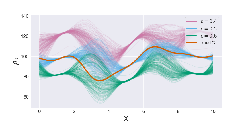
This figure reveals the strong negative correlation between the wave speed and the mean of \(\rho_0\). This correlation between the two parameters can be understood from the solution of the PDE for flow as described earlier: \(q(x, t) = c\rho_0(x-ct)\). If the wave speed \(c\) increases, the mean of \(\rho_0\) must decrease to keep flow at the detectors approximately constant (and vice-versa). Since the pCN sampler does not account for this correlation structure, large pCN updates are highly unlikely to be accepted and the sampler is slow. In contrast, FES adapts to the correlation structure, eliminating the major bottleneck in the sampling.

Discussion

Bob Carpenter’s explanation of why ensemble methods fail in high dimensions is of course correct: ensemble methods will fail in high dimensions because interpolating and extrapolating between points will fall outside the typical set. However high dimensional spaces are not all high dimensional in the same way.

Throughout the post Bob uses a high dimensional Gaussian (ie: a doughnut) to illustrate when ensemble methods fail. Indeed, we statistician often use the Gaussian distribution to illustrate ideas or simplify reasoning. For example, a standard line of thinking when developing a new method might be to argue: “in the case of everything being Gaussian our method becomes exact..”. This makes sense because Gaussians are easy to manipulate and pop up everywhere because of the central limit theorem.

However, it can be unhelpful to build our mental models of difficult concepts - such as high dimensional distributions - solely on Gaussians. Indeed, difficult sampling problems are hard precisely because they are not Gaussian. This is similar to the problem of using model organsisms in biology to learn about humans. So in a way, Gaussians are the fruit flies of statistics.

High-dimensional distributions

There are many ways in which high dimensional distributions might be different from a spherical Gaussian which we can use to help with sampling. One way is that there might exist a low dimensional subspace that represents most of the “interesting bits” of the posterior. The rest of the space (the complementary subspace) is then relatively unaffected by the likelihood and therefore acts like the prior. This is similar to the idea behind PCA where the data mainly lives on a low dimensional subspace.

In our inverse problem involving functional parameters, the prior gives a natural way to find this low dimensional subspace. This is because the Gaussian process prior imposes a lot of structure on the parameter which allows the infinite dimensional problem to be well posed.

To be perfectly clear: if you have gradients, you should use them! In the function space setting there are many gradient-based methods that will do much better than this ensemble method, such as function space versions of HMC and MALA as well as dimensionality reduction methods. However in our paper we rather focused on the setting where gradients were unavailable. So gradient-free samplers are about doing the best you can with limited information.

Conclusion

Making MCMC work is about finding a good parametrisation. HMC uses Hamilton’s equations to find a natural parametrisation (ie: level sets). However, this can still break down with difficult geometries and another reparametrisation might be necessary.

If you don’t have gradients then ensemble methods can be a good solution (example: the emcee package). However if the dimension is too high then these will break down as discussed in Bob Carpenter’s post. Thankfully, this is not the end of the road for ensemble samplers! You’ll then need to think about your problem to identify natural groupings of parameters to apply your gradient-free sampler to. In this post I went over a practical way to do this in the case of infinite-dimensional inverse problems, yielding a simple but powerful gradient-free ensemble sampler defined on function spaces.

Thanks to Robert J Webber and Bob Carpenter for useful feedback on this post