This post is the first of a two-part series on early Monte Carlo methods from the 1940s and 1950s. Although Monte Carlo methods had been previously hinted at (for example Buffon’s needle), these methods only started getting serious attention in the 1940s with the development of fast computers. In 1949 a conference on Monte Carlo was held in Los Angeles in which the participants - many of them legendary mathematicians, physicists, and statisticians - shared their work involving Monte Carlo methods. It can be enlightening to review this research today to understand what issues these researchers were grappling with. In this post I’ll give a brief overview on computing and Monte Carlo in the 1940s, and then discuss some of the talks from this 1949 conference. In the next post I’ll go over the classic 1953 paper on the Metropolis sampler and give some details of the MANIAC computer.

Historical context: Monte Carlo in the 1940s

Computing during World War 2

During WW2, researchers at Los Alamos worked on building the atomic bomb which involved solving nonlinear problems (for example in fluid dynamics and neutron transport). As the project advanced they used a series of increasingly powerful computers to do this. Firstly, they used mechanical desk calculators; these were standard calculators at the time, but were slow and unreliable. Then then upgraded to using electro-mechanical business machines which were bulkier but faster. One application was to solve partial differential equations (PDEs). To solve a PDE numerically, one punch card was used to represent each point in space and time, and a set of punch card would represent the state of the system at some point in time. You would pass each set of card through several machines to solve the PDE forward in time. The machines would often break down and would have to be fixed which made doing any calculation laborious. Finally, John von Neumann recommended the scientists use the ENIAC computer which was able to do calculations an order of magnitude faster. You can find more details on computing at Los Alamos in this report by Francis Harlow and Nick Metropolis.

Monte Carlo in the 40s

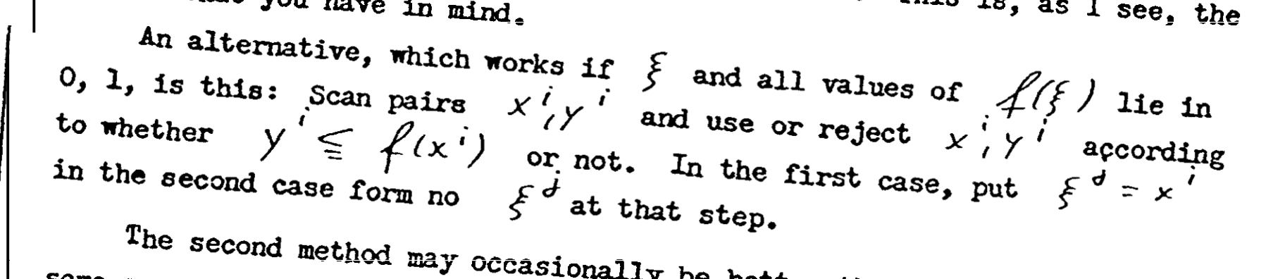
A well known story about early Monte Carlo methods is about Stan Ulam playing solitaire while he was ill (see this article by Roger Eckhardt for more details). He wondered what the probability was of winning at solitaire if you simply laid out a random configuration. After trying to calculating this mathematically, he then considered laying out many random configurations and simply counting how many of them were successful. This is a simple example of the Monte Carlo method: using randomness to estimate a non-random quantity. Ulam - along with John von Neumann - then starting thinking how to apply this method to solve problems involving neutron diffusions. Von Neumann was important in developing new Monte Carlo methods and new computers as well as giving legitimacy to these new fields; that such a well respected scientist was interested in these things helped these fields become respectable among other scientists. At that time Monte Carlo methods mainly seemed to spread by word of mouth. For example we can see in figure 1 an extract from a letter written by von Neumann to Ulam in 1947 describing rejection sampling. You can see more of the letter in Eckhardt’s article.

The 1949 Conference on Monte Carlo

In 1949 a conference was held in Los Angeles to discuss recent research on Monte Carlo. This was the first time a lot of these methods were published: the speakers gave talks and some of these were written up in a report. The attendees of this conference included a lot of famous mathematicians, statisticians, and physicists such as von Neumann, Tukey, Householder, Wishart, Neyman, Feller, Harris, and Kac. The speakers introduced such sampling methods as the rejection sampler, the middle square method, and splitting schemes for rare event sampling (these three methods were actually suggested by von Neumann). There were also talks about applications in such areas as particle and nuclear physics as well as statistical mechanics.

We’ll now focus on two of the talks, both presenting techniques invented by von Neumann.

the Middle Square Method

Von Neumann introduced the Middle Square method, which was a way to quickly generate pseudorandom numbers. A standard way at the time of obtaining random numbers was to generate a list of uniform random numbers using some kind of physical process, then use that list of random numbers in calculations. However when using computers such as the ENIAC or MANIAC, reading this list into the computer was much too slow. It was therefore necessary to generate these random numbers on the fly, even if that meant obtaining random samples of lower quality.

The method works as follows:

• Start from an integer with \(n\) digits (with \(n\) even):
• Square the number
• If the square has \(2n-1\) digits, add a leading zero (to the left of it) so that the new number has \(n\) digits
• keep the \(n\) digits in the middle of the number.

For example, if we start from the seed \(a_0 = 20\) (2 digits) the algorithm runs as follows:

• \(20^2=0400\), so \(a_1=40\)
• \(40^2=1600\), so \(a_2 = 60\)
• Then \(a_i = 60\) for \(i>2\). Here the process has converged and will only generate the number \(60\) from now on.

So we notice that we need to use a carefully chosen large seed (namely, at least 10 digits). If we don’t choose a good seed the numbers might quickly converge and the algorithm will keep on generating the same number for ever. A lot of careful work was therefore done on finding good seeds and doing statistical tests on the generated numbers to assess their quality. One of the talks in the conference discusses some tests done on this algorithm (see talk number 12 by George Forsythe).

Obviously today we have much better PRNGs, so we should use these modern methods and not the middle square process. But it is interesting to see some of the early work on PRNGs.

Rejection sampling

Von Neumann also introduce rejection sampling (though we saw in figure 1 that he had developed this method several years earlier). This talk is called “Various techniques used in connection with random digits” and a pdf of the talk (without the rest of the conference) can be found here. There also seems to be several dates attributed to this paper (see this stackexchange question about how to properly cite it). In the talk von Neumann first reviews methods used to generate uniform random numbers, then introduces the rejection sampling method and how to use it with a few examples.

Generating uniform random numbers

Von Neumann starts by considering that a physical process (such as nuclear process) can be used to generate high quality random numbers, and that a device could be built that would generate these as needed. However he points out that it would be impossible to reproduce the results (if you need to debug the program for example) as there would be no random seed that would reproduce the same random numbers. He concludes this by saying:

“I think that the direct use of a physical supply of random digits is absolutely inacceptable for this reason and for this reason alone”.

In light of this comment it is interesting to consider how most of modern research code involving random numbers does not keep track of the random seed used, and is therefore not reproducible in this sense (namely, in terms of the realisation of the random variables used).

He then considers generating random numbers using a physical process and printing out the results (this is discussed in another talk in the conference); one can then read in the random numbers to the computer as needed. However he points out that reading in numbers to a computer is the slowest aspect of it (in more modern terms, the problem would be I/O bound).

Finally, he concludes that using arithmetic methods such as the Middle Square method is a nice practical alternative that is both fast and reproducible. However one needs to check whether a random seed will generate random samples of sufficiently high quality. It is here that he famously says:

“Any one who considers arithmetic methods of producing random digits is, of course, in a state of sin. For, as has been pointed out several times, there is no such thing as a random number - there are only methods to produce random numbers, and a strict arithmetic procedure of course is not such a method”

However he takes the very practical approach of recommending we use such arithmetic methods and simply test the generated samples to make sure they are good enough for applications.

The rejection method

In the second part of the talk he considers the problem of generating non-uniform random numbers following some distribution \(f\), namely how to sample \(X \sim f\). This requires using uniformly distributed random numbers (generated using the middle square method for example) and transforming them appropriately.

He first considers using the inverse transform but considers this to be too inefficient. He then introduces the rejection method which is as follows:

• choose a scaling factor \(a \in \mathcal{R^+}\) such that \(af(x) \leq 1\)
• sample \(X, Y \sim \mathcal{U}(0,1)\)
• Accept \(X\) if \(Y \leq af(X)\). Reject otherwise

This last step corresponds to accepting \(X\) with probability \(af(X)\) (which is between \(0\) and \(1\)).

Note that the more modern version of this method considers a general proposal distribution \(g\) (see these lecture notes or any textbook on Monte Carlo):

• let \(l(x) = cf(x)\) be the un-normalised target density (\(f\) is the target, \(c\) is unknown)
• Let \(M \in \mathcal{R}\) be such that \(Mg(x) \geq l(x)\)
• draw \(X \sim g\) and compute: \(r = \frac{l(X)}{Mg(X)}\)
• Accept \(X\) with probability \(r\)

Here we sample \(X\) from a general distribution \(g\) and similarly choose a constant \(M\) such that \(r\) is between \(0\) and \(1\).

Von Neumann then gives several examples such as how to sample from the exponential distribution by computing \(X = - \log(T)\) with \(T \sim Uni(0,1)\). However he considers it silly to generate random number and then plug them into a complicated power series to approximate the logarithm function. He therefore gives an alternative method to transforming the random number \(T\) by only taking simple operations rather than the logarithm.

Round table discussion

The conference ended with a round table discussion led by John Tukey which was documented in section 14 of the report. This was a mix of prepared statements as well as discussions between the participants.

To open the discussion, Leonard Savage read from Plutarch’s Lives; in particular a passage that talks about the siege of Syracuse where Archemedes built machines to defend the city. The passage discusses how Archemedes would not have built these applied machines if the king hadn’t asked him to; these machines were the “mere holiday sport of a geometrician”. Savage then reads about Archytas and Eudoxus - friends of Plato - who developed mathematical mechanics. Plato was apparently not happy about this as this development as:

[mechanics was] destroying the real excellence of geometry by making it leave the region of pure intellect and come within that of the senses and become mixed up with bodies which require much base servile labor.

As a result mechanics was separated from geometry and considered among the military arts. These passages illustrate how applied research and engineering have always been looked down upon by many theoretical researchers. In 1949 Monte Carlo methods and scientific computing were just getting developed so this would indeed have been the case.

Another interested portion of this discussion was given by John Wishart: he pointed out that he was impressed by the interactions between physicists, mathematicians, and statisticians. He considered that the different groups would be able to learn from each other. He also gave stories of how Karl Pearson was very practically minded and would regularly using his “hand computing machine” to solve integral which would help with his research. Pearson and his student Leonard Tippett also generated long lists of random numbers to use in research: these lists would allow them to estimate the sampling distribution of some statistics they were studying.

The rest of the discussion goes over different practical problems and the benefits of having interactions between statistics and physics.

Thoughts on this conference

There seemed to be a strong focus in the conference on practical calculations and experiments. The reading by Leonard Savage at the beginning of the round table discussion seems to reflect the general tone of the conference of being equally comfortable dealing with data and computers as well as maths and theory. Indeed computers at the time were unreliable and regularly broke down so researchers had to be very comfortable with engineering. Von Neumann’s remarks on pseudo random numbers also shows a very practical mindset of using “whatever works” rather than trying to find the “perfect” random number generator.

I also noticed that throughout the talks there was very little mention of Monte Carlo error. Researchers in the 40s had known for a long time about the central limit theorem (CLT), but I didn’t find any explicit link between a Monte Carlo estimate (which is simply an average of samples) and CLT which would have given them an error bar (perhaps this was too obvious to mention?). The main mention of Monte Carlo error I found was by Alston Householder who - in his talk - gives estimates along with the standard errors (page 8). The only other hint of this that I found is the sentence by Ted Harris in the discussion at the end of the conference where he is talking about two different ways of obtaining Monte Carlo samples to estimate some quantity:

… we know that if we do use the second estimate instead of the first and if we do it for long enough then we will come out with exactly the right answer. I am leaving aside the question of the relative variability of the two estimates.

My guess is that either the CLT was too obvious to mention, or that it was hard enough to simply estimate these quantities without also computing error bars. In conclusion, I would recommend reading through some of the talk in the report, in particular the round table discussion.

Conclusion

We saw how Monte Carlo methods took off in the 1940s and that a lot of these new methods and applications were presented in the 1949 conference. In my next post I’ll go over the classic 1953 paper on the Metropolis sampler and give some details of the MANIAC computer.

Thanks to Gael Martin and Christian Robert for useful feedback on this post