Early Monte Carlo methods - Part 2: the Metropolis sampler
This post is the second of a two-part series on early Monte Carlo methods from the 1940s and 1950s. In my previous post I gave an overview of Monte Carlo methods in the 40s and focused on the 1949 conference in Los Angeles. In this post I’ll go over the classic paper Equation of State Calculations by Fast Computing Machines (1953) by Nick Metropolis and co-authors. I’ll give an overview of the paper and its main results and then give some context about how it was written. I’ll then delve into some details of how the MANIAC computer worked to give an idea of what it must have been like to write algorithms such as MCMC on it.
The classic Metropolis sampler paper
Overview of paper
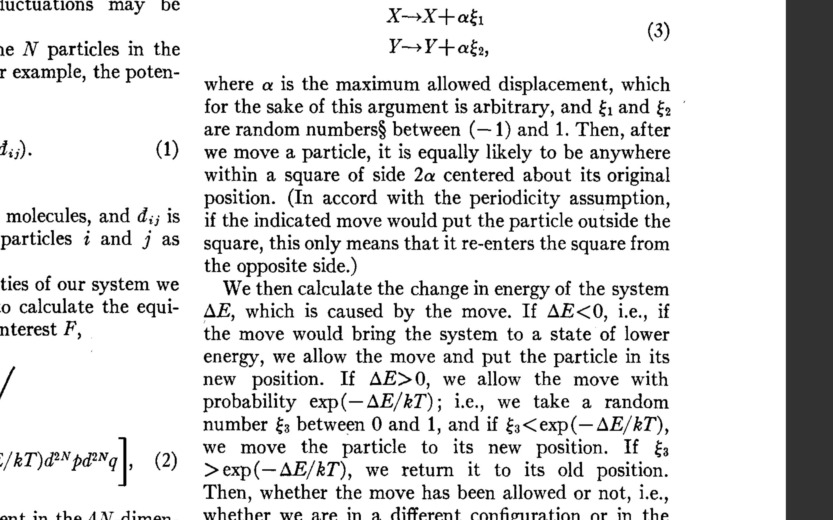
The objective of the paper is to estimate properties (in this case pressure) of a system of interacting particles. The system of study consists of \(N\) particles (which they model as hard disks) in a 2D domain. They mention however that they are working on a 3D problem as well. The potential energy of the system is given by:
\[E = \frac{1}{2} \sum_i^N \sum^N_{j, i\neq j} V(d_{ij})\]Here \(d_{ij}\) is the distance between molecules and \(V\) is the potential between molecules.
It seems that a usual thing to do up to the 1950s to estimate properties for such complicated systems was to approximate them analytically. The paper compares results from MCMC with two standard approximations. They also mention that an alternative method would have to use ordinary Monte Carlo by sampling many particle configurations uniformly and weighing them by their probability (namely by their energy). The problem with this approach is that the weights would all be essentially zero if many particles are involved. Their solution is to rather do the opposite: sample particle configurations based on their probabilities and then take an average (with uniform weights).
After an overview of the problem they introduce the Metropolis sampler: for each particle suggest a new position using a uniform proposal and allow this move with a certain probability. Interestingly, this sampler would be called these days a Metropolis-within-Gibbs sampler or a single-site Metropolis sampler as each particle is updated one at a time. In figure 1 we see the description of the algorithm from the paper.
The algorithm was coded up to run on the MANIAC computer, and took around 3 minutes to update all 242 particles (which is obviously slow by today’s standards). Note that they used the Middle Square method to generate the uniform random numbers in the proposal distribution and the accept-reject step. This random number generator has some issues but is fast and therefore much more convenient than reading in random numbers from a table (this method was introduced in the 1949 conference and is discussed in my previous post).
They then justify the new sampler by giving an argument for how it will converge to the target distribution: they show that the system is ergodic and that detailed balanced is satisfied. Finally, they run experiments and estimate the pressure of a system of particles. They compare the results to two standard analytic approximations, and find that the MCMC results agree with the approximations in the parameter region where they are known to be accurate.
Discussion
This paper explains clearly and simply their new sampler, includes some theoretical justification, and have experiments to show that the method can work in practice. One thing I’m not clear about is that they don’t have access to the ”ground truth”, so it’s not completely clear how we know that the MCMC results are correct. However they do explain how the analytic approximations diverge from the MCMC results exactly in the parameter regions where those approximations are expected to break down.
Another point is that they include some discussion of the Monte Carlo error, but they seem to compute the error using the variance of samples and not correct for the correlation between samples. We now know that we must calculate the integrated autocorrelation time and use it to find the effective sample size. So a nitpick of the paper would be that their Monte Carlo error estimate is too small! We’ll have to wait until Hasting’s paper (see section 2) in 1970 for a rigorous treatment of the variance of estimates from correlated samples.
Finally, they use 16 cycles as burn-in (one cycle involves updating all the particles) and then run 48 to 64 cycles to sample configurations (they run different experiments). I haven’t reproduced this experiment to see the trace plots but intuitively this seems fairly low. However they were limited by the computing power available to them and this must have been enough to get the estimates they were looking for.
An interesting article from 2004 includes the recollections from Marshall Rosenbluth (one of the authors) where he explained the contributions of each of the authors of the paper. It turns out that he and Arianna Rosenbluth (his wife) did most of the work. More specifically, he did the mathematical work, Arianna wrote the code that ran on the MANIAC, August Teller wrote an earlier version of the code, and Edward Teller gave some critical suggestions about the methodology. Finally, Nick Metropolis provided the computing time; as he was first author the method is therefore named after him. But perhaps a more appropriate name would have been the Rosenbluth algorithm.
MANIAC
A lot of the early Monte Carlo methods were intimately linked with the development of modern computers, such as the ENIAC and the MANIAC 1 (which was used in the Metropolis paper). It therefore makes sense to look into some detail how these computers worked to see what it must have been like to write code for them. We’ll look into some sections from the MANIAC’s documentation to get a taste for how this computer worked.
Historical context
The MANIAC computer was a step in a series of progressively faster and more reliable computers. Its construction started in 1946, was operational in 1952 (just in time for the 1953 Metropolis paper), and shut down in 1958. It was used to work on a range of problems such as PDEs, integral equations, and stochastic processes. It was succeeded by the MANIAC II (built in 1957) and the MANIAC III (1964) which were faster and easier to use. To give some context, Fortran came out in 1957, Lisp in 1958, and Cobol in 1959. So code written for the MANIAC was not at all portable; you had to learn how to program for this specific machine.
Arithmetic
We start by looking at the introduction (often a nice place to start) of the documentation (page 6 in the pdf). We find that numbers are represented as binary digits (which was to be expected). Note that they use the word bigit to mean a binary digit; it’s perhaps a shame that this term didn’t stick. I’ll use it throughout the rest of the post as I like it.
The storage capacity of the MANIAC is:
- 1 sign bigit
- 39 numerical bigits
We then put a decimal point before the first numerical bigit. The number 0.2 (in decimal) would then be represented on the MANIAC as 0.11 (binary). Note that this means that numbers can only be between \(-1\) and \(1\). So if your program will generate numbers outside this range you must either scale the numbers before doing the calculations or adjust the magnitudes of numbers on the fly.
Negative numbers
We now consider negative numbers on the MANIAC (page 7 of the pdf). The natural thing to do to generate a negative number would be to have the sign bigit be 0 for a positive number and 1 for a negative number (or vice versa). But the MANIAC represents the negative of the number \(x\) as the complement of \(x\) with respect to \(2\), namely:
As \(0 < x < 1\) we have \(1 < c < 2\). This means that the sign bigit will always be 1 for negative numbers, and that all the numerical bigits of \(c\) will be the bigits of \(x\) flipped.
To illustrate this, suppose that \(x = -.101110101...011\) (in binary). This means that it’s representation on the MANIAC will be c = 1.010001010...101. Note that the sign bigit is 1, and that all the digits are flipped with the exception of the last one (which is always 1). You can check that this is the case by calculating the difference \(2-x\) in binary, namely 10.000...000 - 0.101110101...011.
This way of representing negative numbers may feel convoluted, but taking the complement of a number is easy to do on the MANIAC; you simply flip the numerical bigits and change the sign bigit.
Subtraction
The benefits of writing negative numbers in this weird way become even more apparent when we consider subtraction. To subtract \(b\) from \(a\) you simply add \(a\) to the complement of \(b\). This means that \(a-b\) becomes \(a + (2-b)\) (assuming that \(a,b>0\)).
Let’s check that this works for \(a,b>0\). We have to consider two cases: \(a>b\) and \(a<b\).
first case: \(a>b\)
The first case to consider is when \(a>b\). As both numbers are between \(0\) and \(1\) we have:
\[\begin{align} 0 &< a - b < 1 \\ 2 &< 2 + (a - b) < 3 \end{align}\]We represent the number \(2 + (a-b)\) in binary as 10.<numerical bigits>... However the leftmost bigit is outside the capacity of the computer so is dropped (which subtracts \(2\) from the result), and you end up with the correct number: \(a-b\).
second case: \(a<b\)
In this case we have:
\[\begin{align} -1 &< a - b < 0 \\ 1 &< 2 + (a - b) < 2 \\ 1 &< 2 - (b - a) < 2 \end{align}\]The term \(2- (b-a)\) is simply the complement of \(b-a\), namely “negative” \(b-a\). This is also exactly the result we wanted!
The other cases - as recommended in the documentation (see figure 2 below) - are left as exercises to the reader.

So subtraction reduces to flipping some bigits and doing addition.
Modular arithmetic
Finally, this way of doing subtraction doesn’t feel so weird anymore if we think about modular arithmetic. For example if we are working modulo \(10\) and want to subtract \(3\) from a number, we can simply add the complement of \(3\) which is \(10-3=7\). Namely:
\[\begin{align} - 3 &\equiv 7 \hspace{2mm} (10) \\ x - 3 &\equiv x + 7 \hspace{2mm} (10) \\ \end{align}\]This is exactly how the MANIAC does subtraction, but modulo \(2\) rather than \(10\).
Writing programs
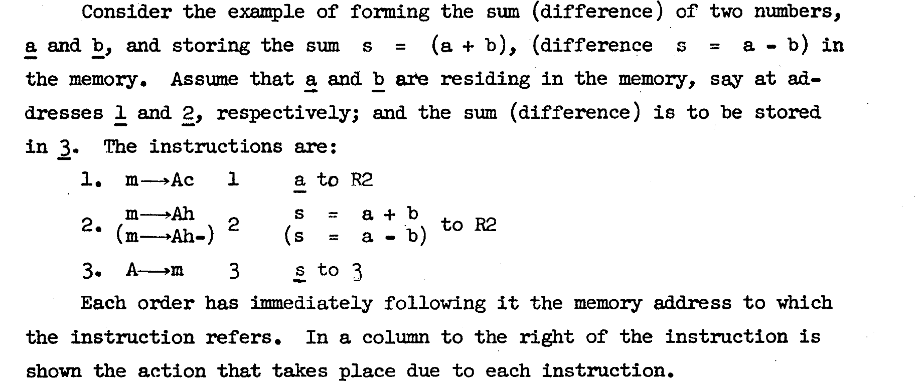
The programmer had to be very comfortable with this way of representing numbers and be able to write complicated numerical methods such as MCMC or PDE solvers. They would describe every step of the program on a “computing sheet” before representing them on a punch card which was finally fed into the MANIAC. Figure 3 shows a sample from the documentation which describes the instructions need to implement subtraction.
The documentation then goes on to describe more complicated operations, such as taking square roots, as well as the basics of MANIAC’s internal design.
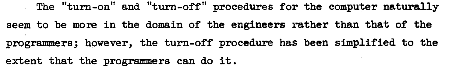
In conclusion, coding was complicated and required working with engineers as the machines broke down regularly. The only built-in operators were (+), (-), (*), (%), and inequality/equalities. Figure 4 (below) is a sample from the documentation and shows how this computer was an improvement from previous versions: it was so simple that even a programmer could turn in on and off!
Conclusion
The development of Monte Carlo methods took off in the 1940s, and this work was closely tied to the progress of computing. The usual applications at the time were in particle and nuclear physics, fluid dynamics, and statistical mechanics. In this post we went over the classic 1953 paper on the Metropolis sampler and went over some details of the MANIAC computer. We saw how the computers used in scientific research were powerful (for the era), but were complicated machines that required a lot of patience and detailed knowledge to use.
Thanks to Gael Martin and Christian Robert for useful feedback on this post